Blog Layout

MAY CONTAIN BAD ASS CONTENT: ANALYST DISCRETION IS ADVISED

Basic Census Analytics with Alteryx

James Smith • Aug 13, 2020

US Census has details on 230,000 areas in the US

Now that you have connected to the census data, you can begin to explore it in huge detail using Alteryx. In this post, we can use the spatial tools to find local information about any area or zip code in the US.

The following link contains the workflow in Alteryx.  It is based on a connection to the safegraph data set in the data exchange post.  


If you have followed the previous posts and setup a file connection, all you need to do is go to Options-->Advanced Options-->Workflow Dependencies and replace the my connection file with the file you setup to connect to your instance.

From here, I'll walk through the basic workflow and then we can do a deeper dive into how this data set is structured so we can ask more questions.

WORKFLOW WALKTHROUGH

The top leg of the workflow starts with the census questions.  This contains all the questions on the 2010 census.  We first filter the questions to get questions related to population  "TABLE_ID" LIKE B0110%e%.   Snowflake uses standard SQL syntax meaning that the % symbol is a wildcard.  This says give me all tables starting with B0110 then that have an "e" and then any other value after that.   B0110 are all the population related questions and the e means estimate.  You can also get m meaning margin of error.


On the bottom leg of the workflow we are going to connect to the responses for the B01 table (this has the answers to each question) - the top leg has the questions themselves.    Here we can select the questions we are interested in.   In the example it's just total population.  But you could easily add other questions like male population between the ages of 22 to 24 by selecting B01001E10, as an example.


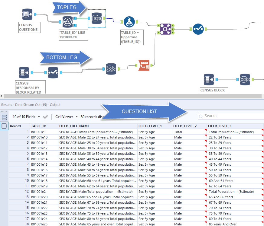
After each leg, we will use the datastream out tool to bring the result set into Alteryx.  On the bottom leg, we need a simple pivot to get the question_id as a row instead of a field (header).  Joining will bring the question into context of the answer.  Then with the select tool we just choose the question context and now we can an answer by census block.

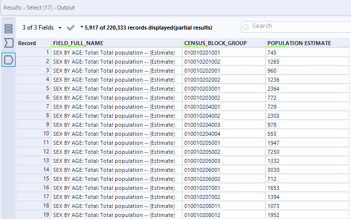
Now a census block isn't very useful to us without context, but there is a census block metadata table as well in the data source, which has details on each census block.  That table for reference is "METADATA_CBG_GEOGRAPHIC_DATA"


Downloading this data and joining it back by census group gives you population as well as coordinates and the land area and water area for each census group.   


Adding a create points tool from the spatial object bar enables us to transform this data into a map object visible through any browse tool.


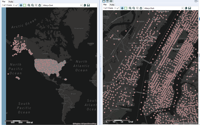
Now that is absurdly detailed!!    And remember we have details on this level for over 7,000 individual questions from the census.     In future posts we will show how to build this up to aggregate trade areas around your specific locations of interest.

17 Dec, 2020
Anyone who follows me knows how much I love the combination of Alteryx and Snowflake. Alteryx provides a logic layer that enables any analyst to manipulate data and Snowflake provides the scale needed to get some amazing insights across large data sets. However, I have found there were always a few things missing. The Alteryx In-DB tools, while comprehensive, cannot do everything. There are some gaps (most notably - ahem - any Alteryx product managers reading this - simple Pivot or Unpivot tools in-DB). There is also a lot of functionality like changing warehouses, schemas or databases that cannot be easily done from within Alteryx.
02 Nov, 2020
In our previous post, we discussed why d emand forecasting matters and how an accurate demand forecast can mathematically and quantitatively improve your service level and/or inventory levels (cost). Now it is time to focus on the biggest uncertainty of them all . Time. Advanced forecasting algorithms can help eliminate uncertainty through reducing variables that are “unknown” by understanding relationships at a scale that no human could comprehend. This helps turn the seemingly “unknown” in to a “known”. As we stated earlier, advances in math and cloud computing make finding these relationships much easier and can be computed almost instantaneously. However, the element of time is a tricky compounding factor. Even little unknowns become big over time as time compounds all errors and introduces more uncertainties. The most certainty you have is in the precise moment you make an estimate. When you look ahead 1 day, 1 week or even 1-month (as most corporate S&OP) cycles still do – then you must start to rely less and less on facts and more and more on assumptions. Assumptions mean uncertainty and uncertainty means cost. There are loads of examples of this. When I lived in Florida, every September during hurricane season , we would get the dreaded cone of uncertainty any time a hurricane formed. As below shows , the further out you get, the expected position gets wider. By day 5 - the uncertainty stretched over 500 miles – hardly accurate enough to do any planning of significance  .
By James Smith 14 Sep, 2020
You cannot go far these days without hearing about data science, digital transformation or AI. This is especially true in the supply chain discipline. However, when taking it back to basics, what AI, ML and Data Science are really doing are solving mathematical equations that are hardly new. These equations are just trying to optimize a series of variables to minimize cost and maximize service – something supply chain professionals have been doing for decades. So what has changed? Cloud Computing and Cloud Storage! Cloud Computing is enabling supply chain professionals to perform more math, faster. Cheap Storage is providing the ability to store more data about products and environmental variables which gives more fuel for the math to solve.
Share by: